Building LLM part 2

In this blog, we will go through chapter 2 of “Build a Large Language Model From Scratch” by Sebastian Raschka. This chapter is about working with text. It goes over preparing text for LLMs, splitting text into word and subword tokens, byte pair encoding, sliding window for dataloader sampling, and converting tokens into embeddings.

Image generated from copilot.

Here is an outline:

• Intorduction
• Tokenizing text
  • Preprocessing text to split words and special characters.
  • Creating vocab
  • Encoding and decoding text using the vocab.
  • Adding special tokens for encoding/decoding (such as <|unk|>, <|endoftext|>)
• Creating dataloader
  • Parameters to play with: batch_size, max_length, stride, shuffle, drop_last, num_workers
• What is an embedding?
  • Talk about embedding briefly in LLMs.
  • Why use embedding?
  • Examples of using embeddings in other fields.
  • Pros and cons of using embedding.
  • Creating embedding
  • Positional embedding
• Byte pair encoding

Introduction

In the last blog, we went over an introduction to Large Language Models (LLMs). In this blog, we will go over preparing text data for the training. First, we tokenize the text into numbers. Second, we build the dataloader. Lastly, we turn it into embeddings. As a bonus, we will also go over byte pair encoding in the end. Materials for this blog are from chapter 2 of “Build a Large Language Model From Scratch” by Sebastian Raschka with some adjustments. And the images and code are from the book and the author’s github repo.

Tokenizing Text

There are many ways to tokenize text, but we will keep it simple. We will only split the text into words, punctuations, and special characters and then convert them into numbers. This is called encoding. On the other hand, decoding is converting the numbers back into the text. We will use a dictionary to map each token to a number, and this will become a vocabulary. We will also add some special tokens to the vocabulary, such as <|unk|> for unknown tokens. Then we can test our encoding and decoding.

Preprocessing text

In preprocessing step, we will split the text into words, punctuations, and special characters. We will use the re module to split the text into tokens.

import re
text = "The cat sat on the mat!"
res = re.split(r'(\s)', text)
res

['The', ' ', 'cat', ' ', 'sat', ' ', 'on', ' ', 'the', ' ', 'mat!']

Let’s also split on special characters and punctuation.

res = re.split(r'([,.:;?_!"()\']|--|\s)', text)
res

['The', ' ', 'cat', ' ', 'sat', ' ', 'on', ' ', 'the', ' ', 'mat', '!', '']

We can remove the white space using list comprehension.

res = re.split(r'([,.:;?_!"()\']|--|\s)', text)
[o.strip() for o in res if o.strip()]

['The', 'cat', 'sat', 'on', 'the', 'mat', '!']

Let’s use a bigger text.

raw_text = '''The cat sat on the mat! She saw a red ball rolling by, and jumped up to chase it. "Meow?" she wondered, looking at the ball that was now under the table @ 123 Main Street.'''
raw_text

'The cat sat on the mat! She saw a red ball rolling by, and jumped up to chase it. "Meow?" she wondered, looking at the ball that was now under the table @ 123 Main Street.'

prep = re.split(r'([,.:;?_!"()\']|--|\s)', raw_text)
prep = [o.strip() for o in prep if o.strip()]
prep[:15]

['The',
 'cat',
 'sat',
 'on',
 'the',
 'mat',
 '!',
 'She',
 'saw',
 'a',
 'red',
 'ball',
 'rolling',
 'by',
 ',']

Creating vocab

Now that we have preprocessed the text, we can create a vocabulary. The vocabulary is a mapping from each token to a number. We will use a dictionary to store the mapping.

all_words = sorted(set(prep))
vocab_size = len(all_words)
vocab_size

38

vocab = {token:integer for integer,token in enumerate(all_words)}
vocab

{'!': 0,
 '"': 1,
 ',': 2,
 '.': 3,
 '123': 4,
 '?': 5,
 '@': 6,
 'Main': 7,
 'Meow': 8,
 'She': 9,
 'Street': 10,
 'The': 11,
 'a': 12,
 'and': 13,
 'at': 14,
 'ball': 15,
 'by': 16,
 'cat': 17,
 'chase': 18,
 'it': 19,
 'jumped': 20,
 'looking': 21,
 'mat': 22,
 'now': 23,
 'on': 24,
 'red': 25,
 'rolling': 26,
 'sat': 27,
 'saw': 28,
 'she': 29,
 'table': 30,
 'that': 31,
 'the': 32,
 'to': 33,
 'under': 34,
 'up': 35,
 'was': 36,
 'wondered': 37}

We also need a way to reverse the mapping.

rev_vocab = {i:s for s,i in vocab.items()}
rev_vocab

{0: '!',
 1: '"',
 2: ',',
 3: '.',
 4: '123',
 5: '?',
 6: '@',
 7: 'Main',
 8: 'Meow',
 9: 'She',
 10: 'Street',
 11: 'The',
 12: 'a',
 13: 'and',
 14: 'at',
 15: 'ball',
 16: 'by',
 17: 'cat',
 18: 'chase',
 19: 'it',
 20: 'jumped',
 21: 'looking',
 22: 'mat',
 23: 'now',
 24: 'on',
 25: 'red',
 26: 'rolling',
 27: 'sat',
 28: 'saw',
 29: 'she',
 30: 'table',
 31: 'that',
 32: 'the',
 33: 'to',
 34: 'under',
 35: 'up',
 36: 'was',
 37: 'wondered'}

Encoding and Decoding

Now that we have the vocabulary, we can encode and decode text.

tokens = [vocab[s] for s in prep]
tokens[:10]

[11, 17, 27, 24, 32, 22, 0, 9, 28, 12]

And here is how we decode. We first turn it back into a list of tokens, then join them together.

strs = [rev_vocab[i] for i in tokens]
strs[:10]

['The', 'cat', 'sat', 'on', 'the', 'mat', '!', 'She', 'saw', 'a']

strs = ' '.join(strs)
strs

'The cat sat on the mat ! She saw a red ball rolling by , and jumped up to chase it . " Meow ? " she wondered , looking at the ball that was now under the table @ 123 Main Street .'

There are extra spaces in the decoded text. Let’s remove them using re.sub.

re.sub(r'\s+([,.?!"()\'])', r'\1', strs)

'The cat sat on the mat! She saw a red ball rolling by, and jumped up to chase it." Meow?" she wondered, looking at the ball that was now under the table @ 123 Main Street.'

raw_text

'The cat sat on the mat! She saw a red ball rolling by, and jumped up to chase it. "Meow?" she wondered, looking at the ball that was now under the table @ 123 Main Street.'

Let’s compare it to the original text. It looks pretty good, except it." Meow?". It should be it. "Meow?". But it’s not a big deal. We can fix it later.

Putting it all together, here is SimpleTokenizerV1 class that we can use to encode and decode text.

class SimpleTokenizerV1:
    def __init__(self, vocab):
        self.str_to_int = vocab
        self.int_to_str = {i:s for s,i in vocab.items()}
    
    def encode(self, text):
        preprocessed = re.split(r'([,.:;?_!"()\']|--|\s)', text)
        preprocessed = [item.strip() for item in preprocessed if item.strip()]
        return [self.str_to_int[s] for s in preprocessed]
        
    def decode(self, ids):
        text = " ".join([self.int_to_str[i] for i in ids])
        text = re.sub(r'\s+([,.?!"()\'])', r'\1', text)
        return text

tokenizer = SimpleTokenizerV1(vocab)
tokenizer.encode(raw_text)[:10]

[11, 17, 27, 24, 32, 22, 0, 9, 28, 12]

tokens[:10]

[11, 17, 27, 24, 32, 22, 0, 9, 28, 12]

tokenizer.decode(tokenizer.encode(raw_text))

'The cat sat on the mat! She saw a red ball rolling by, and jumped up to chase it." Meow?" she wondered, looking at the ball that was now under the table @ 123 Main Street.'

Adding special tokens

There are some special tokens such as <|unk|> that we need to add to the vocabulary. We will add them to the vocabulary and update the tokenizer.

Special tokens in LLMs serve specific functional purposes and are typically added to the vocabulary with reserved IDs (usually at the beginning). Here are the most common ones:

1. [UNK] or <|unk|> - Used for unknown tokens not in vocabulary
2. [PAD] - Used to pad sequences to a fixed length in a batch
3. [BOS] or <|startoftext|> - Marks the beginning of a sequence
4. [EOS] or <|endoftext|> - Marks the end of a sequence
5. [SEP] - Used to separate different segments of text (common in BERT)
6. [CLS] - Special classification token (used in BERT-like models)
7. [MASK] - Used for masked language modeling tasks

These tokens are crucial because they: - Help models understand sequence boundaries - Enable batch processing of variable-length sequences - Support specific training objectives - Handle out-of-vocabulary words

There are many special tokens. They help the model understand the sequence boundaries, handle out-of-vocabulary words, and support specific training objectives. However, GPT-2 only used <|endoftext|> because it could also be used for padding. This token is also used for separating documents, such as wikipedia articles. It signals the model that the article ended.

Our tokenizer fails when it encounters a token that is not in the vocabulary. Let’s add a special token <|unk|> to the vocabulary and update the tokenizer.

tokenizer.encode("wassup yo")

---------------------------------------------------------------------------
KeyError                                  Traceback (most recent call last)
Cell In[18], line 1
----> 1 tokenizer.encode("wassup yo")

Cell In[14], line 9, in SimpleTokenizerV1.encode(self, text)
      7 preprocessed = re.split(r'([,.:;?_!"()\']|--|\s)', text)
      8 preprocessed = [item.strip() for item in preprocessed if item.strip()]
----> 9 return [self.str_to_int[s] for s in preprocessed]

Cell In[14], line 9, in <listcomp>(.0)
      7 preprocessed = re.split(r'([,.:;?_!"()\']|--|\s)', text)
      8 preprocessed = [item.strip() for item in preprocessed if item.strip()]
----> 9 return [self.str_to_int[s] for s in preprocessed]

KeyError: 'wassup'

len(vocab)

38

vocab['<|endoftext|>'] = len(vocab)
vocab['<|unk|>'] = len(vocab)
vocab

{'!': 0,
 '"': 1,
 ',': 2,
 '.': 3,
 '123': 4,
 '?': 5,
 '@': 6,
 'Main': 7,
 'Meow': 8,
 'She': 9,
 'Street': 10,
 'The': 11,
 'a': 12,
 'and': 13,
 'at': 14,
 'ball': 15,
 'by': 16,
 'cat': 17,
 'chase': 18,
 'it': 19,
 'jumped': 20,
 'looking': 21,
 'mat': 22,
 'now': 23,
 'on': 24,
 'red': 25,
 'rolling': 26,
 'sat': 27,
 'saw': 28,
 'she': 29,
 'table': 30,
 'that': 31,
 'the': 32,
 'to': 33,
 'under': 34,
 'up': 35,
 'was': 36,
 'wondered': 37,
 '<|endoftext|>': 38,
 '<|unk|>': 39}

Now, we can update our encoder to use special tokens.

class SimpleTokenizerV2:
    def __init__(self, vocab):
        self.str_to_int = vocab
        self.int_to_str = {i:s for s,i in vocab.items()}
    
    def encode(self, text):
        prep = re.split(r'([,.:;?_!"()\']|--|\s)', text)
        prep = [item.strip() for item in prep if item.strip()]
        prep = [item if item in self.str_to_int else "<|unk|>" for item in prep]
        return [self.str_to_int[s] for s in prep]
        
    def decode(self, ids):
        text = " ".join([self.int_to_str[i] for i in ids])
        text = re.sub(r'\s+([,.?!"()\'])', r'\1', text)
        return text

tokenizer = SimpleTokenizerV2(vocab)

text1 = "Wassup yo, how's it going?"
text2 = "The cat sat on the mat! She saw a red ball rolling by, and jumped up to chase it. \"Meow?\" she wondered"
text = " <|endoftext|> ".join((text1, text2))
print(text)

Wassup yo, how's it going? <|endoftext|> The cat sat on the mat! She saw a red ball rolling by, and jumped up to chase it. "Meow?" she wondered

tokenizer.encode(text)[:10]

[39, 39, 2, 39, 39, 39, 19, 39, 5, 38]

tokenizer.decode(tokenizer.encode(text))

'<|unk|> <|unk|>, <|unk|> <|unk|> <|unk|> it <|unk|>? <|endoftext|> The cat sat on the mat! She saw a red ball rolling by, and jumped up to chase it." Meow?" she wondered'

Great. We can encode and decode without getting an error from the vocabulary. GPT-2 did not use the <|unk|> token. Instead, it used a byte pair encoding method to handle out-of-vocabulary words. We will go over byte pair encoding in the end.

Creating dataloader

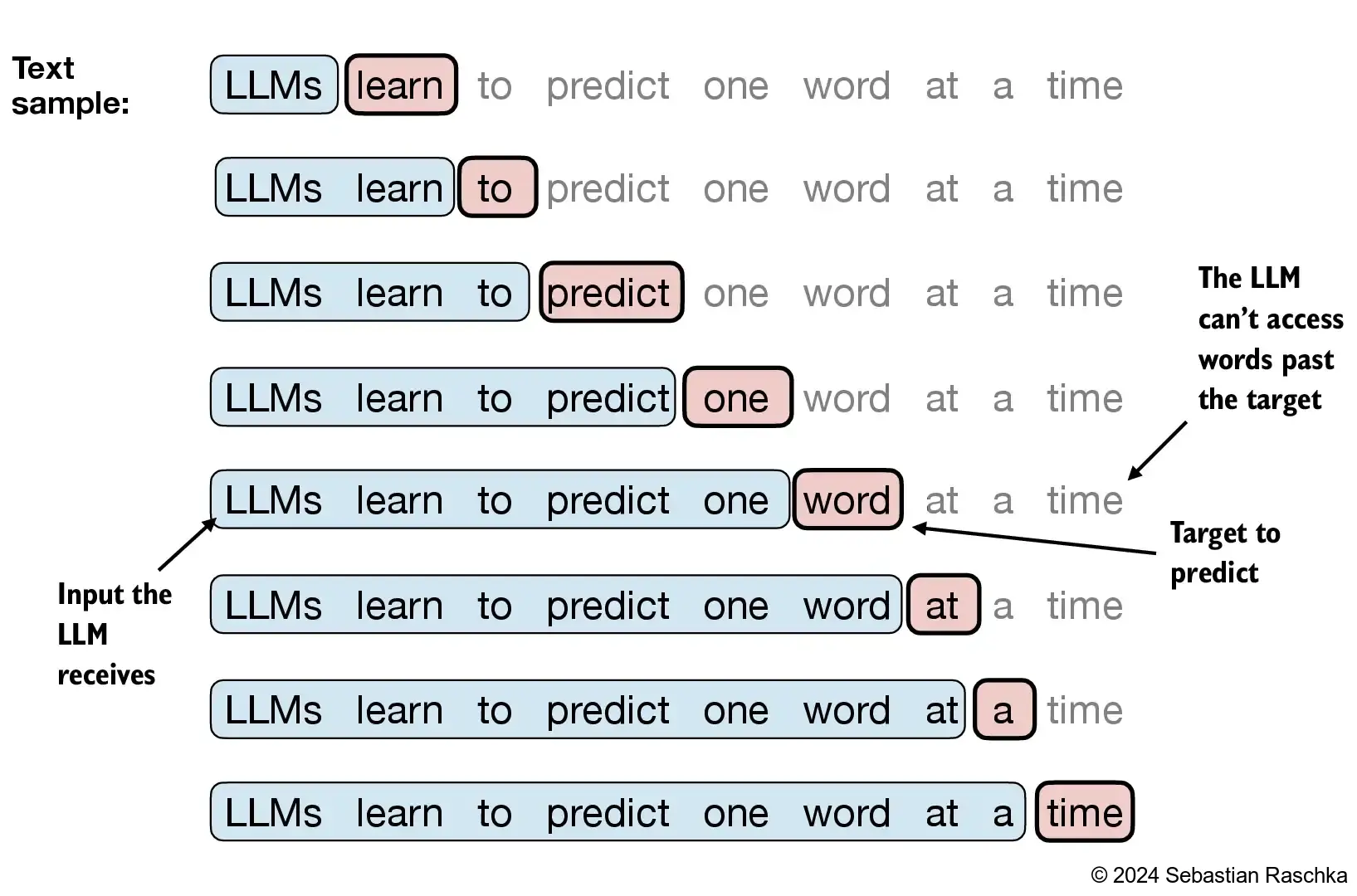
Now that we have tokenized the text, we can create a dataloader. Using dataloader is an easy way to turn the encoded text into batches of data. In each batch, we have a sequence of tokens for x and another for y. The x sequence is the input, and the y sequence is the output. The y sequence is the same as the x sequence, but shifted by one token. This is because we want the model to predict the next token given the previous tokens. The dataloader is also responsible for batching the data and shuffling it.

tokens = tokenizer.encode(raw_text)
tokens[:10]

[11, 17, 27, 24, 32, 22, 0, 9, 28, 12]

We set the context_size as 4. This means x and y are 4 tokens long. This is only a toy example, but in GPT, context size is way bigger. For example, GPT-2 has a context size of 1024. This means that the model can see up to 1024 tokens in the past. This is why GPT-2 is so good at generating text. It can see the context of the text and generate text that is more coherent. However, longer context size means more memory usage.

context_size = 4

x = tokens[:context_size]
y = tokens[1:context_size+1]

print(f"x: {x}")
print(f"y:      {y}")

x: [11, 17, 27, 24]
y:      [17, 27, 24, 32]

When training, this is what the model sees as x and y:

for i in range(1, context_size+1):
    x = tokens[:i]
    y = tokens[i]

    print(x, "---->", y)

[11] ----> 17
[11, 17] ----> 27
[11, 17, 27] ----> 24
[11, 17, 27, 24] ----> 32

For more readability, decoded version is here:

for i in range(1, context_size+1):
    x = tokens[:i]
    y = tokens[i]

    print(tokenizer.decode(x), "---->", tokenizer.decode([y]))

The ----> cat
The cat ----> sat
The cat sat ----> on
The cat sat on ----> the

Let’s create a pytorch dataset. As long as we have __len__ and __getitem__, we can use it with pytorch dataloader.

class GPTDatasetV1:
    def __init__(self, txt, tokenizer, max_length, stride):
        self.input_ids = []
        self.target_ids = []

        token_ids = tokenizer.encode(txt, allowed_special={"<|endoftext|>"})

        # Use a sliding window to chunk the book into overlapping sequences of max_length
        for i in range(0, len(token_ids) - max_length, stride):
            input_chunk = token_ids[i:i + max_length]
            target_chunk = token_ids[i + 1: i + max_length + 1]
            self.input_ids.append(torch.tensor(input_chunk))
            self.target_ids.append(torch.tensor(target_chunk))

    def __len__(self): return len(self.input_ids)

    def __getitem__(self, idx): return self.input_ids[idx], self.target_ids[idx]

We will use tiktoken library to get an encoding from gpt2. We’ve pretty much looked at everything in this code except stride. max_length is the context size. stride is the number of tokens to skip when creating the next sequence. For example, if max_length is 4 and stride is 2, then the next sequence will start 2 tokens after the previous sequence. This is to avoid having the same sequence in the dataset multiple times. This is a common technique in NLP. It is called sliding window. It is also called sliding window attention. By avoiding the same sequence multiple times, we can reduce the size of the dataset. This is important because we want to use as much data as possible to train the model. It also reduces overfitting.

import tiktoken
import torch
from torch.utils.data import DataLoader

ds = GPTDatasetV1(raw_text, tiktoken.get_encoding("gpt2"), max_length=10, stride=5)
len(ds)

7

def create_dataloader_v1(txt, batch_size=4, max_length=256, 
                         stride=128, shuffle=True, drop_last=True,
                         num_workers=0):
    tokenizer = tiktoken.get_encoding("gpt2")
    dataset = GPTDatasetV1(txt, tokenizer, max_length, stride)
    return DataLoader(
        dataset,
        batch_size=batch_size,
        shuffle=shuffle,
        drop_last=drop_last,
        num_workers=num_workers
    )

Dataloader returns x and y. Let’s take a look at what stride does in a dataloader. Here is a simple example of batch_size of 1 and stride 1.

dataloader = create_dataloader_v1(raw_text, batch_size=1, max_length=4, stride=1, shuffle=False)
next(iter(dataloader))

[tensor([[ 464, 3797, 3332,  319]]), tensor([[3797, 3332,  319,  262]])]

Let’s look at batch_size of 2. Both x and y are 2 sequences long. The first sequence is the same as the previous example. The second sequence is the next sequence in the text.

dataloader = create_dataloader_v1(raw_text, batch_size=2, max_length=4, stride=1, shuffle=False)
next(iter(dataloader))

[tensor([[ 464, 3797, 3332,  319],
         [3797, 3332,  319,  262]]),
 tensor([[3797, 3332,  319,  262],
         [3332,  319,  262, 2603]])]

When we increase the stride to 2, the second sequence is 2 tokens after the first sequence. This is because we skipped 2 tokens when creating the second sequence. Instead of starting the second x with 3797, we start with 3332.

dataloader = create_dataloader_v1(raw_text, batch_size=2, max_length=4, stride=2, shuffle=False)
next(iter(dataloader))

[tensor([[ 464, 3797, 3332,  319],
         [3332,  319,  262, 2603]]),
 tensor([[3797, 3332,  319,  262],
         [ 319,  262, 2603,    0]])]

When we have the same stride and max_length, we can see that the second sequence is the same as the first sequence. This is because we skipped 4 tokens when creating the second sequence. Now, there is no overlap between the x sequences and y sequences.

dataloader = create_dataloader_v1(raw_text, batch_size=2, max_length=4, stride=4, shuffle=False)
next(iter(dataloader))

[tensor([[ 464, 3797, 3332,  319],
         [ 262, 2603,    0, 1375]]),
 tensor([[3797, 3332,  319,  262],
         [2603,    0, 1375, 2497]])]

Note that we also have drop_last parameter. This is to drop the last batch if it is smaller than batch_size. This is important during training because it can cause loss spikes.

What Are Embeddings?

An embedding is a way to represent words or phrases as vectors of numbers. These vectors capture the semantic meaning of the words, allowing us to perform mathematical operations on them. For example, we can calculate the distance between two words to see how similar they are. Embeddings are used in many NLP tasks, such as machine translation, text classification, and question answering. They are also used in recommendation systems, image recognition, and other machine learning tasks. Embeddings are a powerful tool for understanding and processing text data.

For example, in this space: - “Cat” and “dog” might be close together because they’re both pets - “Run” and “sprint” would be nearby as they’re similar actions - “Hot” might be positioned opposite to “cold” - “King”, “queen”, “prince”, and “princess” would form a cluster showing both their royal relationships and gender differences

In modern LLMs like GPT-2, each token (word or subword) is represented by a vector of 768 numbers, while larger models like GPT-3 use even bigger vectors (2048 or more dimensions). These numbers aren’t randomly assigned - they’re learned during training to capture meaningful relationships between words.

Why Do We Need Embeddings?

Traditional one-hot encoding represents each word as a vector of zeros with a single ‘1’, where the vector length equals vocabulary size. For a 50,000-word vocabulary, each word requires a 50,000-dimensional vector! This approach has several major problems:

1. Inefficiency:
   • Massive storage requirements
   • Sparse representations (mostly zeros)
   • Computationally expensive to process
2. No Semantic Information:
   • “cat” and “kitten” are as different as “cat” and “motorcycle”
   • No way to measure word similarity
   • No capture of analogies or relationships

Embeddings solve these problems by: 1. Dense Representation: - Using much smaller vectors (768 vs 50,000 dimensions) - Every dimension carries meaningful information - Efficient storage and computation

2. Semantic Relationships:
   • Similar words have similar vectors
   • Enable amazing arithmetic: king - man + woman ≈ queen
   • Capture multiple types of relationships:
     • Semantic (car/automobile)
     • Syntactic (run/running)
     • Conceptual (France/Paris :: Japan/Tokyo)
3. Learning and Adaptation:
   • Embeddings improve during model training
   • Can capture domain-specific meanings
   • Transfer learning from one task to another
4. Mathematical Operations:
   • Calculate similarity using cosine distance
   • Find analogies through vector arithmetic
   • Cluster related concepts together

Embeddings Beyond Language Models

The power of embeddings extends far beyond just processing text. The same fundamental concept - representing complex objects as dense vectors in high-dimensional space - has revolutionized many fields:

1. Recommendation Systems:
   • Netflix maps both users and movies into the same embedding space
   • User embeddings capture viewing preferences and habits
   • Movie embeddings represent genre, style, mood, and other features
   • Similarity between vectors predicts what you might like to watch
   • Even time-of-day and viewing context can be embedded
2. Computer Vision:
   • Images are embedded into high-dimensional spaces
   • Similar images cluster together automatically
   • Enables powerful features like:
     • Face recognition
     • Object detection
     • Image similarity search
     • Style transfer
   • Transfer learning from pre-trained vision models
3. Bioinformatics:
   • Protein sequences represented as embeddings
   • Captures complex biochemical properties
   • Predicts protein folding and interactions
   • Helps in drug discovery
   • Enables rapid searching of similar compounds
4. Audio Processing:
   • Spotify embeds songs based on:
     • Musical features (tempo, key, instruments)
     • Listening patterns
     • Cultural context
     • User behavior
   • Voice recognition systems use embeddings
   • Sound classification and similarity detection
5. Graph Networks:
   • Social networks embed users and relationships
   • Knowledge graphs embed concepts and connections
   • Traffic networks embed locations and routes
   • Fraud detection systems embed transaction patterns

Creating Embeddings in Practice

Creating embeddings involves several key components and considerations:

1. The Embedding Layer:

embedding_dim = 768  # typical size
vocab_size = 50257  # GPT-2 vocabulary size
embedding_layer = nn.Embedding(vocab_size, embedding_dim)

2. Initialization Strategies:
   • Random initialization
   • Pre-trained embeddings (Word2Vec, GloVe)
   • Xavier/Glorot initialization
   • Custom initialization based on domain knowledge
3. Training Approaches:
   • End-to-end with model
   • Separate pre-training
   • Fine-tuning existing embeddings
   • Frozen pre-trained embeddings
4. Advanced Techniques:
   • Subword tokenization
   • Contextual embeddings
   • Multi-modal embeddings
   • Hierarchical embeddings

The Position Problem

Position information is crucial in language understanding, but transformers are inherently position-agnostic. Here’s how we solve this:

1. Learned Positional Embeddings:
   • Model learns position representations
   • Can capture common patterns
   • More flexible but needs training
   • Used in models like GPT
2. Sinusoidal Embeddings:
   • Fixed mathematical patterns
   • Uses sine and cosine functions
   • Different frequencies for different dimensions
   • Original transformer approach
   • No training required
   • Can extrapolate to longer sequences
3. Relative Positional Embeddings:
   • Encode relative distances between tokens
   • Better for certain tasks
   • More computationally intensive
   • Used in modern architectures like T5
4. Hybrid Approaches:
   • Combining different types
   • Task-specific adaptations
   • Novel architectural innovations

Trade-offs and Challenges

The use of embeddings, while powerful, comes with important considerations and challenges:

1. Training Data Requirements:
   • Need massive amounts of quality data
   • Data must be representative and balanced
   • Domain-specific data often required
   • Poor quality data leads to poor embeddings
   • Data cleaning and preprocessing crucial
2. Computational Costs:
   • Training embeddings is resource-intensive
   • Large memory requirements
   • GPU/TPU hardware often necessary
   • Inference time can be significant
   • Storage costs for large embedding tables
3. Bias and Fairness:
   • Embeddings inherit biases from training data
   • Can amplify societal prejudices
   • Gender, racial, and cultural biases common
   • Debiasing techniques available but imperfect
   • Ethical considerations in deployment
4. Technical Challenges:
   • Choosing optimal embedding dimension
   • Handling out-of-vocabulary words
   • Dealing with rare words/tokens
   • Managing embedding table size
   • Updating embeddings efficiently
5. Performance Trade-offs:
   • Accuracy vs. computation speed
   • Memory usage vs. embedding size
   • Training time vs. model quality
   • Generalization vs. specialization
   • Real-time requirements vs. model complexity

The Future of Embeddings

1. Architectural Innovations:
   • More efficient embedding architectures
   • Sparse embedding techniques
   • Dynamic embedding sizes
   • Adaptive embedding strategies
   • Novel initialization methods
2. Multi-modal Developments:
   • Cross-modal embeddings
   • Universal embeddings across domains
   • Joint learning of different modalities
   • Transfer learning improvements
   • Domain adaptation techniques
3. Efficiency Improvements:
   • Compression techniques
   • Quantization methods
   • Pruning strategies
   • Distributed embedding systems
   • Hardware-specific optimizations
4. Ethical Considerations:
   • Better debiasing techniques
   • Fairness-aware embeddings
   • Interpretable embeddings
   • Privacy-preserving methods
   • Robust evaluation metrics
5. Emerging Applications:
   • Quantum computing embeddings
   • Neuromorphic hardware adaptation
   • Edge device implementations
   • Real-time embedding updates
   • Federated learning approaches
6. Research Directions:
   • Theoretical understanding improvements
   • Formal mathematical frameworks
   • Stability and robustness studies
   • Scaling laws investigation
   • Novel training objectives

The field of embeddings continues to be a crucial area of research and development in machine learning, with new breakthroughs and applications emerging regularly. As we better understand their properties and capabilities, we can expect to see even more innovative uses across various domains.

To learn more about embeddings, please refer to the following resources: - Google’s tutorial on word embeddings, document search, and applications: https://github.com/google/generative-ai-docs/tree/main/site/en/gemini-api/tutorials

Tip: word embeddings size with multiples of 64 have hardware optimization.

Using Embeddings

Let’s create embeddings with pytorch. We will use a simple example.

token_ids = torch.tensor([2,1,0])
token_ids

tensor([2, 1, 0])

vocab_size = 3
output_dim = 4

torch.manual_seed(42)
emb = torch.nn.Embedding(vocab_size, output_dim)
emb

Embedding(3, 4)

emb.weight

Parameter containing:
tensor([[ 0.3367,  0.1288,  0.2345,  0.2303],
        [-1.1229, -0.1863,  2.2082, -0.6380],
        [ 0.4617,  0.2674,  0.5349,  0.8094]], requires_grad=True)

An embedding layer has weights defined by the vocab size and the output dimension. The weights are normally distributed with mean of 0 and standard deviation of 1. These weights are learnable parameters. With these embedding layer, we can convert the token ids into embeddings by simply calling the embedding layer with the token ids.

# First embedding
emb(torch.tensor([0]))

tensor([[0.3367, 0.1288, 0.2345, 0.2303]], grad_fn=<EmbeddingBackward0>)

# Second embedding
emb(torch.tensor([1]))

tensor([[-1.1229, -0.1863,  2.2082, -0.6380]], grad_fn=<EmbeddingBackward0>)

We can also simply select using an index.

emb.weight[0]

tensor([0.3367, 0.1288, 0.2345, 0.2303], grad_fn=<SelectBackward0>)

Or we can select multiple embeddings at once in whatever order we want.

emb(torch.tensor([1,0]))

tensor([[-1.1229, -0.1863,  2.2082, -0.6380],
        [ 0.3367,  0.1288,  0.2345,  0.2303]], grad_fn=<EmbeddingBackward0>)

emb(token_ids)

tensor([[ 0.4617,  0.2674,  0.5349,  0.8094],
        [-1.1229, -0.1863,  2.2082, -0.6380],
        [ 0.3367,  0.1288,  0.2345,  0.2303]], grad_fn=<EmbeddingBackward0>)

One-hot encoding

An older way to do this is using one hot encoding.

We can manually do one hot encoding

params = torch.nn.Parameter(emb.weight)
params

Parameter containing:
tensor([[ 0.3367,  0.1288,  0.2345,  0.2303],
        [-1.1229, -0.1863,  2.2082, -0.6380],
        [ 0.4617,  0.2674,  0.5349,  0.8094]], requires_grad=True)

onehot = torch.nn.functional.one_hot(token_ids)
onehot

tensor([[0, 0, 1],
        [0, 1, 0],
        [1, 0, 0]])

onehot.float()@params

tensor([[ 0.4617,  0.2674,  0.5349,  0.8094],
        [-1.1229, -0.1863,  2.2082, -0.6380],
        [ 0.3367,  0.1288,  0.2345,  0.2303]], grad_fn=<MmBackward0>)

We can also use a linear layer

linear = torch.nn.Linear(vocab_size, output_dim, bias=False)
linear.weight = torch.nn.Parameter(emb.weight.T)
linear.weight

Parameter containing:
tensor([[ 0.3367, -1.1229,  0.4617],
        [ 0.1288, -0.1863,  0.2674],
        [ 0.2345,  2.2082,  0.5349],
        [ 0.2303, -0.6380,  0.8094]], requires_grad=True)

linear(onehot.float())

tensor([[ 0.4617,  0.2674,  0.5349,  0.8094],
        [-1.1229, -0.1863,  2.2082, -0.6380],
        [ 0.3367,  0.1288,  0.2345,  0.2303]], grad_fn=<MmBackward0>)

Using torch.nn.Embedding is the most efficient way to convert token ids into embeddings. It’s faster and more memory-efficient than using one-hot encoding or a linear layer.

Positional Embeddings

Positional embeddings are added to the token embeddings to encode the position of the token in the sequence. This is because transformers do not have any inherent sense of order. There are two main types of positional embeddings: relative positional embeddings and absolute positional embeddings.

• Relative positional embeddings

Relative positional embeddings encode the distance between tokens. This is useful because the model can learn to pay attention to tokens that are close to each other. However, relative positional embeddings are not as efficient as absolute positional embeddings.

• Absolute positional embeddings

Absolute positional embeddings encode the absolute position of the token in the sequence. This is useful because the model can learn to pay attention to tokens that are in certain positions. However, absolute positional embeddings are not as flexible as relative positional embeddings. It can be difficult to change the size of the context length of the model because it was fixed during the training.

Usually, these embeddings are added to the token embeddings.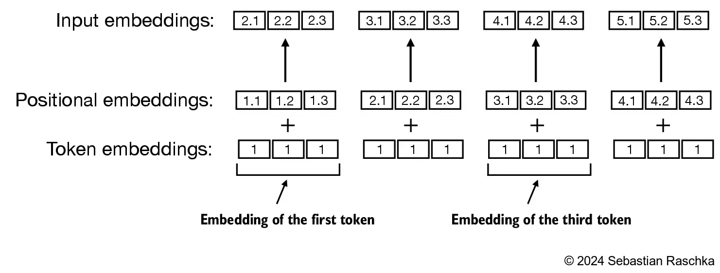

Let’s create absolute positional embeddings for simplicity. GPT-2 also used this. We have token_ids and emb from before.

token_ids

tensor([2, 1, 0])

emb

Embedding(3, 4)

Let’s get token embeddings again.

token_emb = emb(token_ids)
token_emb

tensor([[ 0.4617,  0.2674,  0.5349,  0.8094],
        [-1.1229, -0.1863,  2.2082, -0.6380],
        [ 0.3367,  0.1288,  0.2345,  0.2303]], grad_fn=<EmbeddingBackward0>)

Positional embedding is another embedding layer with the same output dimension as the token embedding layer. The input dimension is the context length. The context length is the maximum length of the sequence that the model can handle. In this case, we will use a context length of 3. And output size is 4. Since vocab size and output size are the same, we can use the same embedding layer for both token and positional embeddings.

emb2 = torch.nn.Embedding(3, 4)
emb2

Embedding(3, 4)

pos_emb = emb2(torch.arange(3))
pos_emb

tensor([[-0.7658, -0.7506,  1.3525,  0.6863],
        [-0.3278,  0.7950,  0.2815,  0.0562],
        [ 0.5227, -0.2384, -0.0499,  0.5263]], grad_fn=<EmbeddingBackward0>)

Finally, we can get the input embedding for the model by adding the token embeddings and the positional embeddings.

inp_emb = token_emb + pos_emb
inp_emb

tensor([[-0.3042, -0.4833,  1.8875,  1.4957],
        [-1.4506,  0.6086,  2.4897, -0.5818],
        [ 0.8594, -0.1095,  0.1846,  0.7567]], grad_fn=<AddBackward0>)

To learn more about positional embeddings, please refer to the following resources: - A blog on Rotary Position Encoding (ROPE) by Akash Nain: https://aakashkumarnain.github.io/posts/ml_dl_concepts/rope - Reformer paper: https://arxiv.org/pdf/2104.09864

Byte pair encoding (BPE)

Byte pair encoding (BPE) is a data compression technique that is used to create a vocabulary of subword units. It was a bit confusing for me to understand this because I forgot about bytes, hexdecimal, ASCII, and UTF-8. However, the algorithm is very simple. BPE is useful because it allows the model to handle out-of-vocabulary words. It works by iteratively merging the most frequent pair of bytes in the text. This process is repeated until the desired vocabulary size is reached. The resulting vocabulary consists of the most frequent subword units in the text.

The book does not cover details of BPE, but bpe-from-scratch is included in the github. This version focuses on education purposes and skips some steps, such as converting the text into bytes. To learn more about bpe, I recommend minbpe by Karpathy.

How BPE works

Briefly, this is how to train BPE:

1. Vocabulary is initialized with first 256 ASCII characters.
2. Text is converted into bytes.
3. Until vocabulary size is reached:
   • Count the frequency of each pair of bytes in the text.
   • Merge the most frequent pair of bytes into a single byte.
   • Add the new byte to the vocabulary.

That’s it. BPE is a simple and effective way to create a vocabulary of subword units. It is used in many NLP models, including GPT-2, GPT-3, and BERT. I was planning on explaining BPE in more detail, but I think it is better to leave it as an exercise for the reader. Maybe I will write a blog on it in the future with some information about bytes, hexadecimal digits, ASCII, UTF-8, and such. Of course it is not necessary to understand BPE, but they are related and are fun to learn about.