Resnet

Author

galopy

Published

December 4, 2023

In this blog, we will talk about Residual network (Resnet). Resnet came from Deep Residual Learning for Image Recognition by Kaiming He et al. We have seen Kaiming/He initialization from the author before.

Data

Figure 1 from Deep Residual Learning for Image Recognition.

Import libraries and Data Setup

from google.colab import drive
drive.mount('/content/drive')

!pip -q install torcheval
!pip -q install datasets
Mounted at /content/drive
/content/drive/MyDrive/Colab Notebooks
     ━━━━━━━━━━━━━━━━━━━━━━━━━━━━━━━━━━━━━━━━ 179.2/179.2 kB 2.0 MB/s eta 0:00:00
     ━━━━━━━━━━━━━━━━━━━━━━━━━━━━━━━━━━━━━━━━ 521.2/521.2 kB 3.6 MB/s eta 0:00:00
     ━━━━━━━━━━━━━━━━━━━━━━━━━━━━━━━━━━━━━━━━ 115.3/115.3 kB 11.4 MB/s eta 0:00:00
     ━━━━━━━━━━━━━━━━━━━━━━━━━━━━━━━━━━━━━━━━ 134.8/134.8 kB 13.5 MB/s eta 0:00:00
import torch

from miniai.datasets import *
from miniai.conv import *
from miniai.learner import *
from miniai.activations import *
from miniai.init import *
from miniai.sgd import *
# from miniai.resnet import *
import pickle,gzip,math,os,time,shutil,torch,matplotlib as mpl,numpy as np,matplotlib.pyplot as plt
import fastcore.all as fc
from collections.abc import Mapping
from pathlib import Path
from operator import attrgetter,itemgetter
from functools import partial
from copy import copy
from contextlib import contextmanager

import torchvision.transforms.functional as TF,torch.nn.functional as F
from torch import tensor,nn,optim
from torch.utils.data import DataLoader,default_collate
from torch.nn import init
from torch.optim import lr_scheduler
from torcheval.metrics import MulticlassAccuracy
from datasets import load_dataset,load_dataset_builder

from miniai.datasets import *
from miniai.conv import *
from miniai.learner import *
from miniai.activations import *
from miniai.init import *
from miniai.xtras import *
from fastcore.test import test_close

torch.set_printoptions(precision=2, linewidth=140, sci_mode=False)
torch.manual_seed(1)

import logging
logging.disable(logging.WARNING)

set_seed(42)
dls = get_dls()
dt = dls.train
xb,yb = next(iter(dt))
xb.shape,yb[:10]
(torch.Size([1024, 1, 28, 28]), tensor([5, 7, 4, 7, 3, 8, 9, 5, 3, 1]))
metrics = MetricsCB(accuracy=MulticlassAccuracy())
astats = ActivationStats(fc.risinstance(GeneralRelu))
cbs = [DeviceCB(), metrics, ProgressCB(plot=False), astats]
iw = partial(init_weights, leaky=0.1)
act_gr = partial(GeneralRelu, leak=0.1, sub=0.4)

Resnet

Before we get into the code, let’s see what resent is and why it works conceptually.

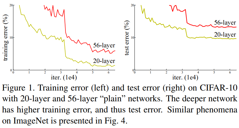
In the paper, the team found that deep neural networks performed worse than shallow neural networks. In theory, a deeper net should capture more details and perform better. The problem persisted even when they built the deep neural net from the shallow one appended with additional layers. If appended layers did nothing, the deeper net should perform as well as the shallower net. However, these appended layers hampered the training.

Resblock

Figure 2. from Deep Residual Learning for Image Recognition

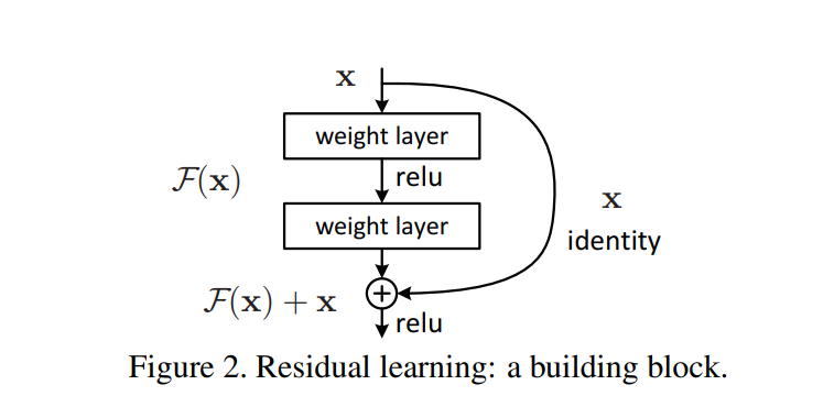
Instead of appending layers at the end of the shallow net, they used deep residual learning framework. So, there is an input, x, and two layers, F. Applying the layers F on x results in F(x), and we add x to this, resulting in F(x) + x. Here, we can consider F as the additional layers we appended at the end of the shallow net in the previous approach. However, because we are doing F(x) + x, x acts as a stabilizer. It stabilizes F(x) if there is no improvement. x is called identity and stabilizes the training.

Let’s get into the code. We can define F(x) + x as a ResBlock. We define _conv_block, which has two convolutional layers. The first layer changes the input from ni to nf with stride one, and the second layer uses the given stride without activation.

def _conv_block(ni, nf, ks=3, stride=2, act=nn.ReLU, norm=None, bias=None):
    return nn.Sequential(conv(ni, nf, ks, 1, act, norm, bias),
                         conv(nf, nf, ks, stride, False, norm, bias))

In ResBlock, we use nn.AvgPool2d if stride is two and a convolutional layer with kernel size one to match the shape of x and F(x) when there is a stride and/or ni is different from nf.

class ResBlock(nn.Module):
    def __init__(self, ni, nf, ks=3, stride=2, act=nn.ReLU, norm=None, bias=None):
        super().__init__()
        self.conv = _conv_block(ni, nf, ks, stride, act, norm, bias)
        self.pool = fc.noop if stride==1 else nn.AvgPool2d(2, ceil_mode=True)
        self.eye = fc.noop if ni==nf else conv(ni, nf, ks=1, stride=1, act=False)
        self.act = act()

    def forward(self, x):
        return self.act(self.conv(x) + self.eye(self.pool(x)))
def get_model(act=nn.ReLU, nfs=[8,16,32,64,128,256], norm=None):
    layers = [ResBlock(1, 8, stride=1, act=act, norm=norm)]
    layers += [ResBlock(nfs[i], nfs[i+1], act=act, norm=norm) for i in range(len(nfs)-1)]
    return nn.Sequential(*layers, conv(nfs[-1],10, act=None, norm=False, bias=True),
                         nn.Flatten()).to(def_device)

Model Summary

By looking into the input and output shapes from the layers, we can look at layers and their shapes quickly. By using the summary, it is more convenient to build a model.

def print_shapes(hook, m, inp, outp):
    print(m.__class__.__name__, inp[0].shape, outp.shape)
model = get_model()
learn = TrainLearner(model, dls, F.cross_entropy, cbs=[SingleBatchCB(), DeviceCB()])
with Hooks(model, print_shapes) as h: learn.fit(1)
ResBlock torch.Size([1024, 1, 28, 28]) torch.Size([1024, 8, 28, 28])
ResBlock torch.Size([1024, 8, 28, 28]) torch.Size([1024, 16, 14, 14])
ResBlock torch.Size([1024, 16, 14, 14]) torch.Size([1024, 32, 7, 7])
ResBlock torch.Size([1024, 32, 7, 7]) torch.Size([1024, 64, 4, 4])
ResBlock torch.Size([1024, 64, 4, 4]) torch.Size([1024, 128, 2, 2])
ResBlock torch.Size([1024, 128, 2, 2]) torch.Size([1024, 256, 1, 1])
Sequential torch.Size([1024, 256, 1, 1]) torch.Size([1024, 10, 1, 1])
Flatten torch.Size([1024, 10, 1, 1]) torch.Size([1024, 10])

We can patch it into the Learner and use it as a class method.

@fc.patch
def summary(self:Learner):
    res = '|Module|Input|Output|Num params|\n|--|--|--|--|\n'
    num = 0
    def _f(hook, m, inp, outp):
        nonlocal res, num
        num_params = sum(o.numel() for o in m.parameters())
        res += f'|{m.__class__.__name__}|{tuple(inp[0].shape)}|{tuple(outp.shape)}|{num_params}|\n'
        num += num_params
    with Hooks(self.model, _f) as hook: self.fit(1, train=False, cbs=[SingleBatchCB()])
    print('Total number of params:', num)
    if fc.IN_NOTEBOOK:
        from IPython.display import Markdown
        return Markdown(res)
    else:
        print(res)
learn.summary()
Total number of params: 1247362
Module Input Output Num params
ResBlock (1024, 1, 28, 28) (1024, 8, 28, 28) 680
ResBlock (1024, 8, 28, 28) (1024, 16, 14, 14) 3632
ResBlock (1024, 16, 14, 14) (1024, 32, 7, 7) 14432
ResBlock (1024, 32, 7, 7) (1024, 64, 4, 4) 57536
ResBlock (1024, 64, 4, 4) (1024, 128, 2, 2) 229760
ResBlock (1024, 128, 2, 2) (1024, 256, 1, 1) 918272
Sequential (1024, 256, 1, 1) (1024, 10, 1, 1) 23050
Flatten (1024, 10, 1, 1) (1024, 10) 0

GlobalAvgPool

Our model only works on images with 28 by 28 pixels. To use images with higher resolutions, we can use GlobalAvgPool. It simply averages the last two dimensions into one by one. We can then use flatten to remove these dimensions. Then, we can use a linear layer to create an output layer.

class GlobalAvgPool(nn.Module):
    def forward(self, x): return x.mean((-1, -2))
def get_model(act=nn.ReLU, nfs=[8,16,32,64,128,256], norm=None):
    layers = [ResBlock(1, 8, stride=1, act=act, norm=norm)]
    layers += [ResBlock(nfs[i], nfs[i+1], act=act, norm=norm) for i in range(len(nfs)-1)]
    return nn.Sequential(*layers, GlobalAvgPool(), nn.Flatten(), nn.Linear(nfs[-1], 10)).to(def_device)
TrainLearner(get_model(), dls, F.cross_entropy, lr=1).summary()
Total number of params: 1226882
Module Input Output Num params
ResBlock torch.Size([1024, 1, 28, 28]) torch.Size([1024, 8, 28, 28]) 680
ResBlock torch.Size([1024, 8, 28, 28]) torch.Size([1024, 16, 14, 14]) 3632
ResBlock torch.Size([1024, 16, 14, 14]) torch.Size([1024, 32, 7, 7]) 14432
ResBlock torch.Size([1024, 32, 7, 7]) torch.Size([1024, 64, 4, 4]) 57536
ResBlock torch.Size([1024, 64, 4, 4]) torch.Size([1024, 128, 2, 2]) 229760
ResBlock torch.Size([1024, 128, 2, 2]) torch.Size([1024, 256, 1, 1]) 918272
GlobalAvgPool torch.Size([1024, 256, 1, 1]) torch.Size([1024, 256]) 0
Flatten torch.Size([1024, 256]) torch.Size([1024, 256]) 0
Linear torch.Size([1024, 256]) torch.Size([1024, 10]) 2570

Flops

We can also add number of flops into the summary. Number of flops provides the number of operations. The way we calculate flops here is not very accurate, but it still tells us roughly how compute intensive the layer is.

def _flops(x, h, w):
    if x.dim()<3: return x.numel()
    if x.dim()==4: return x.numel()*h*w

Why do we multiply by height and width if dimension is 4? Because whe dimension is 4, it is a convolutional net.

[(o.shape, o.numel()) for o in conv(2, 8).parameters()]
[(torch.Size([8, 2, 3, 3]), 144), (torch.Size([8]), 8)]
[(o.shape, o.numel()) for o in nn.Linear(2, 8).parameters()]
[(torch.Size([8, 2]), 16), (torch.Size([8]), 8)]
@fc.patch
def summary(self:Learner):
    res = '|Module|Input|Output|Num params|Flops|\n|--|--|--|--|--|\n'
    n_params, n_flops = 0, 0
    def _f(hook, m, inp, outp):
        nonlocal res, n_params, n_flops
        num_params = sum(o.numel() for o in m.parameters())
        *_, h, w = outp.shape
        num_flops = sum(_flops(o, h, w) for o in m.parameters())/1e6
        n_params += num_params
        n_flops += num_flops
        res += f'|{m.__class__.__name__}|{tuple(inp[0].shape)}|{tuple(outp.shape)}|{num_params}|{num_flops:.2f}|\n'
    with Hooks(self.model, _f) as hook: self.fit(1, train=False, cbs=[SingleBatchCB()])
    print('Total number of params:', n_params)
    print('Total number of flops:', n_flops)
    if fc.IN_NOTEBOOK:
        from IPython.display import Markdown
        return Markdown(res)
    else:
        print(res)
TrainLearner(get_model(), dls, F.cross_entropy, lr=1).summary()
Total number of params: 1226882
Total number of flops: 4.675826000000001
Module Input Output Num params Flops
ResBlock (1024, 1, 28, 28) (1024, 8, 28, 28) 680 0.51
ResBlock (1024, 8, 28, 28) (1024, 16, 14, 14) 3632 0.70
ResBlock (1024, 16, 14, 14) (1024, 32, 7, 7) 14432 0.70
ResBlock (1024, 32, 7, 7) (1024, 64, 4, 4) 57536 0.92
ResBlock (1024, 64, 4, 4) (1024, 128, 2, 2) 229760 0.92
ResBlock (1024, 128, 2, 2) (1024, 256, 1, 1) 918272 0.92
GlobalAvgPool (1024, 256, 1, 1) (1024, 256) 0 0.00
Flatten (1024, 256) (1024, 256) 0 0.00
Linear (1024, 256) (1024, 10) 2570 0.00

Conclusion

In this blog, we learned about Resnet. As we have seen from the code, it is straightforward. It is conceptually easy to understand why it works as well. We also learned about creating a summary with module names, input and output shapes, number of parameters, and number of flops. It allows us to look at the big picture of the model. It’s also helpful when creating a model and debugging to look at the layers’ shapes.