MNIST Neural Nets

Author

galopy

Published

February 25, 2023

MNIST Project

In this blog, we will use neural networks to train MNIST dataset. We start with using pytorch and integrate fastai in the end.

This is part of Further Research from fastbook chapter 4.

Preparing data

This part is the same as last blog where we created a baseline by calculating means of images.

from fastai.vision.all import *

matplotlib.rc('image', cmap='Greys')
torch.manual_seed(42)

<torch._C.Generator at 0x7fbcfe166830>

path = untar_data(URLs.MNIST)
Path.BASE_PATH = path
path.ls()

100.03% [15687680/15683414 00:00<00:00]

(#2) [Path('training'),Path('testing')]

(path/'training').ls()

(#10) [Path('training/7'),Path('training/8'),Path('training/5'),Path('training/6'),Path('training/9'),Path('training/3'),Path('training/2'),Path('training/0'),Path('training/4'),Path('training/1')]

I looked at the number of files for each number, and they are not the same.

trn_counts = {n: len((path/'training'/str(n)).ls()) for n in range(10)}
trn_counts

{0: 5923,
 1: 6742,
 2: 5958,
 3: 6131,
 4: 5842,
 5: 5421,
 6: 5918,
 7: 6265,
 8: 5851,
 9: 5949}

Since these are paths for images we have to convert them into pytorch tensors. Pytorch provides us with broadcasting ability, which is very fast.

First, we turn image paths into numbers and return as L, which is an upgraded version of list.

def create_images(path):
    return L(PILImage.create(x) for x in path.ls())

ones = create_images(path/'training'/'1')
im1 = ones[0]
im1

We need to turn them into tensors for speed. However, we have to check the shape of tensors to make sure they are broadcastable and the shape is one we’re expecting.

def create_tensor_imgs(imgs):
    "Convert a list of images into a tensor"
    return torch.stack([tensor(im) for im in imgs])

stacked_ones = create_tensor_imgs(ones)
stacked_ones[0].shape

torch.Size([28, 28, 3])

stacked_ones.shape

torch.Size([6742, 28, 28, 3])

Looking at the shape of an image, it is interesting to find out that its shape is [28, 28, 3] (y, x, and color values). I was expecting to see [28, 28] (y and x values) because it is a black and white image. So, let’s see what’s going on here.

array(im1)[10:15, 12:15]

array([[[  0,   0,   0],
        [221, 221, 221],
        [251, 251, 251]],

       [[ 64,  64,  64],
        [236, 236, 236],
        [251, 251, 251]],

       [[127, 127, 127],
        [251, 251, 251],
        [251, 251, 251]],

       [[127, 127, 127],
        [251, 251, 251],
        [251, 251, 251]],

       [[128, 128, 128],
        [253, 253, 253],
        [253, 253, 253]]], dtype=uint8)

So, it is just filled with the same numbers per each row. We just need one column, so we can simply take a mean of last rank.

array(im1)[10:15, 12:15].mean(-1)

array([[  0., 221., 251.],
       [ 64., 236., 251.],
       [127., 251., 251.],
       [127., 251., 251.],
       [128., 253., 253.]])

So, here is the updated version of create_tensor_imgs that calculates a mean so that we can get rid of the last rank of our tensors.

def create_tensor_imgs(imgs):
    "Convert a list of images into a tensor"
    return torch.stack([tensor(im) for im in imgs]).mean(-1, dtype=torch.float)

stacked_ones = create_tensor_imgs(ones)
stacked_ones[0].shape

torch.Size([28, 28])

array(stacked_ones[0])[10:15, 12:15]

array([[  0., 221., 251.],
       [ 64., 236., 251.],
       [127., 251., 251.],
       [127., 251., 251.],
       [128., 253., 253.]], dtype=float32)

Looks good. Now, we want those pixel values to be between 0 and 1 so that it is easier to train neural networks.

def create_tensor_imgs(imgs):
    "Convert a list of images into a tensor"
    return torch.stack([tensor(im) for im in imgs]).mean(-1, dtype=torch.float)/255

stacked_ones = create_tensor_imgs(ones)
array(stacked_ones[0])[10:15, 12:15]

array([[0.        , 0.8666667 , 0.9843137 ],
       [0.2509804 , 0.9254902 , 0.9843137 ],
       [0.49803922, 0.9843137 , 0.9843137 ],
       [0.49803922, 0.9843137 , 0.9843137 ],
       [0.5019608 , 0.99215686, 0.99215686]], dtype=float32)

def stacked_nums(path):
    "Converts path into stacked tensors."
    imgs = create_images(path)
    return create_tensor_imgs(imgs)

stacked_zeros = stacked_nums(path/'training'/'0')
stacked_twos = stacked_nums(path/'training'/'2')
stacked_threes = stacked_nums(path/'training'/'3')
stacked_fours = stacked_nums(path/'training'/'4')
stacked_fives = stacked_nums(path/'training'/'5')
stacked_sixs = stacked_nums(path/'training'/'6')
stacked_sevens = stacked_nums(path/'training'/'7')
stacked_eights = stacked_nums(path/'training'/'8')
stacked_nines = stacked_nums(path/'training'/'9')

We also need test data to check how we’re doing. Without test set, we don’t know whether we are overfitting or not. So, we do the same process we did for test data.

tst_0_tens = stacked_nums(path/'testing'/'0')
tst_1_tens = stacked_nums(path/'testing'/'1')
tst_2_tens = stacked_nums(path/'testing'/'2')
tst_3_tens = stacked_nums(path/'testing'/'3')
tst_4_tens = stacked_nums(path/'testing'/'4')
tst_5_tens = stacked_nums(path/'testing'/'5')
tst_6_tens = stacked_nums(path/'testing'/'6')
tst_7_tens = stacked_nums(path/'testing'/'7')
tst_8_tens = stacked_nums(path/'testing'/'8')
tst_9_tens = stacked_nums(path/'testing'/'9')

tst_tens = L([tst_0_tens, tst_1_tens, tst_2_tens, tst_3_tens, tst_4_tens, 
              tst_5_tens, tst_6_tens, tst_7_tens, tst_8_tens, tst_9_tens])

tst_counts = {n: len((path/'testing'/str(n)).ls()) for n in range(10)}

tst_1_tens.shape, tst_9_tens.shape

(torch.Size([1135, 28, 28]), torch.Size([1009, 28, 28]))

tst_counts

{0: 980,
 1: 1135,
 2: 1032,
 3: 1010,
 4: 982,
 5: 892,
 6: 958,
 7: 1028,
 8: 974,
 9: 1009}

Now, we stack all the training tensors together to create trn_x. And create trn_y with the counts. We zip those together to create a dataset. We also change the shape of tensors from [28, 28] to [784]. This shape is more useful for matrix multiplication we will do later.

trn_x = torch.cat([stacked_zeros, stacked_ones, stacked_twos, 
                   stacked_threes, stacked_fours, stacked_fives, 
                   stacked_sixs, stacked_sevens, stacked_eights, 
                   stacked_nines]).view(-1, 28*28)

trn_y = tensor(list(flatten([[x] * y for x, y in trn_counts.items()])))
trn_dset = list(zip(trn_x, trn_y))

trn_x.shape, trn_y.shape

(torch.Size([60000, 784]), torch.Size([60000]))

show_image(trn_x[50000].view(28,28)), trn_y[50000]

(<AxesSubplot:>, tensor(8))

x, y = trn_dset[0]
x.shape, y.shape

(torch.Size([784]), torch.Size([]))

Training data looks good, so let’s work on the test data.

tst_x = torch.cat([tst_0_tens, tst_1_tens, tst_2_tens, 
                     tst_3_tens, tst_4_tens, tst_5_tens,
                     tst_6_tens, tst_7_tens, tst_8_tens,
                     tst_9_tens]).view(-1, 28*28)

tst_y = tensor(list(flatten([[x] * y for x, y in tst_counts.items()])))
tst_dset = list(zip(tst_x, tst_y))

tst_x.shape, tst_y.shape

(torch.Size([10000, 784]), torch.Size([10000]))

Using neural network

In order to use neural network, we need to initialize parameters, such as weights and bias.

def init_params(size, std=1.0): return (torch.randn(size)*std).requires_grad_()

weights = init_params((28*28, 10))
bias = init_params(1)

We are initializing weights parameter with size (28*28, 10) because 28*28 is the size of our input (reshaped images) and 10 is the size of our output. Why do we return 10 numbers as an output for each image? Because we’re making predictions on each category (from 0 to 9). Out of all those 10 numbers, the biggest number is the model’s guess.

But couldn’t we just output 1 number instead and pick a target based on the range of our output? For instance, we could use sigmoid function to get our output numbers to be between 0 and 1, and if it’s between 0 and 0.1, it is 0, if it’s between 0.1 and 0.2, it is 1, and so on. That’s also a possible approach to this problem.

With those parameters, we will perform matrix multiplications. There are multiple ways to calculate it. One way involves manually transposing a matrix and getting the sum over dimension 1, and another way involves using @ operator, which does all of that for us.

(x*weights.T).sum(dim=1) + bias

tensor([-3.0786,  6.5823, 12.8080, 10.5792, -8.4876, 12.2374,  7.8472, -2.3099,
         2.4677, 16.0547], grad_fn=<AddBackward0>)

x@weights + bias

tensor([-3.0786,  6.5823, 12.8080, 10.5792, -8.4876, 12.2374,  7.8472, -2.3099,
         2.4677, 16.0547], grad_fn=<AddBackward0>)

def linear(xb): return xb@weights + bias

preds = linear(trn_x)
preds

tensor([[ -3.0786,   6.5823,  12.8080,  ...,  -2.3099,   2.4677,  16.0547],
        [ -4.0905,   1.3646,  -1.6264,  ...,  -5.0465,  -8.9219,   5.3742],
        [ -4.6858,  -1.6842,   5.6141,  ...,  -7.0370,   7.6748,   1.3543],
        ...,
        [-15.4864,  -1.8742,  -6.2627,  ...,  -0.1359,  10.1261,  18.8826],
        [-22.5967,   5.1747,  -6.5157,  ...,  -2.5263,  20.9854,  12.2597],
        [-15.9537,  -2.7749,   3.1555,  ...,   5.3508,  11.7086,  13.8179]],
       grad_fn=<AddBackward0>)

So, we know that these numbers represent “socres” for each category. Let’s look at the first prediction.

preds[0]

tensor([-3.0786,  6.5823, 12.8080, 10.5792, -8.4876, 12.2374,  7.8472, -2.3099,
         2.4677, 16.0547], grad_fn=<SelectBackward0>)

From these numbers, the biggest number is 16.0547, which is a prediction for 9. So, this predicted 9. We can use torch.argmax to calculate the maximum index easily.

preds[0].argmax()

tensor(9)

For multiple predictions, we can specify the dimension to be 1.

preds.argmax(dim=1)

tensor([9, 5, 5,  ..., 9, 8, 9])

With predictions on categories, we can calculate accuracy by comparing it to the targets (trn_y).

(preds.argmax(dim=1) == trn_y).float().mean() * 100

tensor(12.0433)

We have about 10% accuracy since we are using randomly initialized parameters to predict.

def acc(pred, targ):
    return (pred.argmax(dim=1) == targ).float().mean() * 100

acc(preds, trn_y)

tensor(12.0433)

Cross entropy loss

In order to improve our accuracy, we have to tweak our weights and biases (parameters). To improve our parameters, we have to use a loss function. Then, we can calculate gradients and use them to update our parameters. Loss functions are just mathematical functions, but they have smooth shapes. This is important because gradients cannot be calculated on sharp edges. Let’s take look at a sigmoid function.

def plot_function(fn, title=None, xmin=-4.1, xmax=4.1):
    x = torch.linspace(xmin, xmax, 20)
    plt.plot(x, fn(x))
    if title: plt.title(title)

plot_function(torch.nn.Sigmoid(), title='Sigmoid function')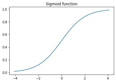

Sigmoid function has no sharp edge, so gradients can be found anywhere. This will also ensure that predictions will be between 0 and 1. We typically use sigmoid function when we try to predict boolean values. For instance, we could use this function for problems like “is it a cat or dog?”

Because we have multiple categories to predict, we use cross entropy loss. Cross entropy loss can be thought of as sigmoid designed for multiple categories. Cross entropy loss is composed of multiple functions. First, we use a softmax function ensures that all numbers are positive and add up to 1. Also, this function takes exponential of all values, so even the slight difference will be magnified. This will result in choosing one class with more confidence. Second, we take the log of the activations we got from softmax. Let’s look at a log function.

plot_function(torch.log, title="Log function", xmin=-0.1, xmax=1)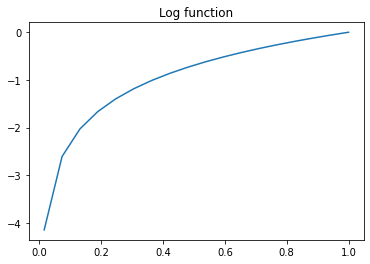

In log function, we get a very big negative value if a number gets closer to 0, and reaches 0 when it gets 1. So, if our activation is close to 0 after softmax, it will be a big negative number after taking a log. This will result in a big gradient. However, if the number is close to 1, it is good enough. So, it will punish numbers that are far off, but forgiving for close numbers. But we still have problems. We still have 10 activation numbers and all of them are negative.

The last function we will use is negative log likelihood, which picks one number from our 10 activations and multiply by -1 to make it a positive value. Although it has log in its name, it actually does not take the log function. We have to do it ourselves. Let’s take a look at how it looks like.

sm_acts = torch.nn.Softmax(dim=1)(preds)
sm_acts[0]

tensor([4.6022e-09, 7.2222e-05, 3.6513e-02, 3.9309e-03, 2.0602e-11, 2.0636e-02,
        2.5585e-04, 9.9276e-09, 1.1795e-06, 9.3859e-01],
       grad_fn=<SelectBackward0>)

log_acts = torch.log(sm_acts)
log_acts[0]

tensor([-19.1967,  -9.5358,  -3.3101,  -5.5389, -24.6057,  -3.8807,  -8.2709,
        -18.4279, -13.6504,  -0.0634], grad_fn=<SelectBackward0>)

trn_y[0]

tensor(0)

torch.nn.NLLLoss()(log_acts[0], trn_y[0])

tensor(19.1967, grad_fn=<NllLossBackward0>)

Notice that we get the same values for the built in cross entropy loss function.

torch.nn.NLLLoss()(log_acts, trn_y)

tensor(14.3907, grad_fn=<NllLossBackward0>)

loss = torch.nn.CrossEntropyLoss()(preds, trn_y)
loss

tensor(14.3907, grad_fn=<NllLossBackward0>)

It’s easier to use the built in function, and it’s also faster.

15.5 ms ± 627 µs per loop (mean ± std. dev. of 7 runs, 100 loops each)

21.7 ms ± 2.67 ms per loop (mean ± std. dev. of 7 runs, 10 loops each)

Calculating gradients

So, we calculated the loss. With loss, we can calculate the gradients by calling backward(). Then, we can take a look at them.

loss.backward()

bias.grad, weights.grad.sum()

(tensor([-9.3132e-09]), tensor(-1.0490e-05))

We can define a function it.

def calc_grad(xb, yb, model):
    "Calculate the gradients"
    preds = model(xb)
    loss = torch.nn.CrossEntropyLoss()(preds, yb)
    loss.backward()
    return loss

weights = init_params((28*28, 10))
bias = init_params(1)

calc_grad(trn_x, trn_y, linear)
weights.grad.mean(), bias.grad.mean()

(tensor(-1.2164e-10), tensor(-9.3132e-09))

After calculating the gradients, we can update our parameters using the gradients. We can multiply parameter’s gradient by any number, which is referred to as a learning rate. If it’s big, it will train faster, and if it’s slow, it will train slower. However, if it’s too big, it cannot train. So, we can try couple numbers and see what works and what doensn’t. After updating, we have to reset the gradients. If we don’t, gradients will keep growing.

weights = init_params((28*28, 10))
bias = init_params(1)
calc_grad(trn_x, trn_y, linear)
bias.grad, weights.grad.sum()

(tensor([-1.3039e-08]), tensor(-9.5367e-07))

calc_grad(trn_x, trn_y, linear)
bias.grad, weights.grad.sum()

(tensor([-2.6077e-08]), tensor(-1.9073e-06))

See how it grew? we have to use zero_() on the gradients. Training _ on functions means in place function.

weights.data -= weights.grad * 10
bias.data -= bias.grad * 10
weights.grad.zero_()
bias.grad.zero_()

tensor([0.])

First training

If we put everything together, this is what it looks like. We will train with the whole data 20 times, which means we are using 20 epochs.

weights = init_params((28*28, 10))
bias = init_params(1)
for _ in range(20):
    calc_grad(trn_x, trn_y, linear)
    weights.data -= weights.grad * 10
    weights.grad.zero_()
    bias.data -= bias.grad * 10
    bias.grad.zero_()
    pred = linear(tst_x)
    print(acc(pred, tst_y))

tensor(20.9500)
tensor(38.9100)
tensor(40.2700)
tensor(48.3800)
tensor(42.6600)
tensor(51.5200)
tensor(45.4200)
tensor(57.6000)
tensor(60.3500)
tensor(62.2100)
tensor(67.2600)
tensor(70.8800)
tensor(75.0300)
tensor(71.8100)
tensor(76.1800)
tensor(82.2500)
tensor(85.1200)
tensor(85.3800)
tensor(85.1700)
tensor(85.1200)

We got over 80% accuracy, which is better tan our baseline using means of images from the last time, which had 66% accuracy. However, we can still make this better.

Minibatches

We updated our parameters after looking at the whole dataset. The MNIST dataset is very small, so it’s not a problem, but dataset can get really big, and it would take a long time to train this way. Another approach to train is update parameters after each image. This is not a good idea either as our model learns about one image at a time, which can lead to overfitting. That’s why we use small batches of data.

dl = DataLoader(trn_dset, bs=256)
xb, yb = first(dl)
xb.shape, yb.shape

(torch.Size([256, 784]), torch.Size([256]))

With fastai’s DataLoader, we will have 256 items per batch. And we will do the same thing for the test set.

tst_dl = DataLoader(tst_dset, bs=256)

def train(lr=1.):
    params = weights, bias
    for xb, yb in dl:
        calc_grad(xb, yb, linear)
        for p in params:
            p.data -= p.grad * lr
            p.grad.zero_()

def validate_epoch(model):
    accs = [acc(model(xb), yb) for xb, yb in tst_dl]
    return round(tensor(accs).mean().item(), 4)

weights = init_params((28*28, 10))
bias = init_params(1)
for _ in range(30):
    train(0.1)
    print(validate_epoch(linear), end='; ')

15.9961; 27.8516; 39.1016; 46.3672; 51.3281; 54.8535; 57.2656; 59.4922; 61.1328; 62.5098; 63.6328; 64.5605; 65.2637; 65.9766; 66.6699; 67.2754; 67.9004; 68.418; 68.9355; 69.3164; 69.6777; 70.0586; 70.3809; 70.625; 70.8789; 71.1328; 71.3379; 71.5039; 71.6602; 71.8262;

Accuracy is not as good as using the whole dataset, but let’s keep trying more things.

Optimizer

We can use pytorch’s torch.nn.Linear instead of our linear. Good thing about using this is that we can get grab parameters easily.

linear_model = torch.nn.Linear(28*28, 10)

w, b = list(linear_model.parameters())
w.shape, b.shape

(torch.Size([10, 784]), torch.Size([10]))

We define a BasicOptim class that has step and zero_grad methods.

class BasicOptim:
    def __init__(self, params, lr=0.01):
        self.params = params
        self.lr = lr
    
    def step(self):
        for p in self.params:
            p.data -= p.grad * self.lr
    
    def zero_grad(self):
        for p in self.params:
            p.grad.zero_()

Optimizer can be used this way. And we can update our train function to use the optimizer.

opt = BasicOptim(list(linear_model.parameters()))

def train(model):
    for xb, yb in dl:
        calc_grad(xb, yb, model)
        opt.step()
        opt.zero_grad()

It’s good to define a function to train a model.

def train_model(epochs, model):
    for _ in range(epochs):
        train(model)
        print(validate_epoch(model))

train_model(20, linear_model)

We can also use fastai’s SGD.

linear_model = nn.Linear(28*28, 10)
opt = SGD(list(linear_model.parameters()), .01)

train_model(20, linear_model)

Also, we can use fastai’s learner. We just need DataLoaders, which combines training dataloaders with test dataloaders. By using learn.fit, we can train easily and get a nice output, too.

dls = DataLoaders(dl, tst_dl)

learn = Learner(dls, nn.Linear(28*28, 10), loss_func=nn.CrossEntropyLoss(), opt_func=SGD, metrics=acc)

learn.fit(20, 0.01)

epoch	train_loss	valid_loss	acc	time
0	1.030682	2.442845	10.260000	00:03
1	0.756178	1.755957	30.840000	00:04
2	0.652057	1.387471	45.750000	00:04
3	0.593682	1.172395	54.570000	00:03
4	0.555542	1.030824	60.259998	00:06
5	0.528407	0.930011	64.510002	00:05
6	0.507978	0.854310	67.820000	00:06
7	0.491943	0.795262	70.309998	00:03
8	0.478946	0.747864	72.440002	00:05
9	0.468138	0.708950	74.440002	00:03
10	0.458963	0.676414	75.860001	00:06
11	0.451041	0.648797	77.139999	00:03
12	0.444104	0.625053	78.199997	00:05
13	0.437957	0.604415	79.160004	00:06
14	0.432457	0.586306	80.010002	00:04
15	0.427493	0.570282	80.739998	00:05
16	0.422980	0.555999	81.290001	00:03
17	0.418851	0.543184	82.040001	00:05
18	0.415051	0.531618	82.360001	00:05
19	0.411538	0.521124	82.720001	00:04

We can improve this accuracy with adding another linear layers and a relu layer. We create a deeper network as long as there’s a relu layer in between each linear layer. Relu layer simply turns negative numbers to 0.

net = nn.Sequential(
    nn.Linear(28*28, 100),
    nn.ReLU(),
    nn.Linear(100, 10)
)

We made a network of layers. Since it is deeper, we have to reduce the learning rate, which results in slower training speed. However, we can train for more epochs. Let’s try training for 100 epochs.

learn = Learner(dls, net, loss_func=nn.CrossEntropyLoss(), 
                opt_func=SGD, metrics=acc)
learn.fit(100, 0.004)

epoch	train_loss	valid_loss	acc	time
0	2.257359	2.186582	28.950001	00:04
1	1.927473	2.062460	16.990000	00:05
2	1.586289	1.925866	19.389999	00:07
3	1.296686	1.757989	29.430000	00:04
4	1.077161	1.585793	37.320000	00:06
5	0.920138	1.439800	42.250000	00:07
6	0.809401	1.322030	45.910000	00:08
7	0.729531	1.226982	48.950001	00:04
8	0.669996	1.148582	52.099998	00:06
9	0.624211	1.082637	54.900002	00:05
10	0.587927	1.026398	57.480000	00:05
11	0.558507	0.977675	59.820000	00:08
12	0.534146	0.934994	62.150002	00:07
13	0.513631	0.897281	63.990002	00:07
14	0.496094	0.863748	65.589996	00:07
15	0.480910	0.833677	66.970001	00:08
16	0.467640	0.806602	68.199997	00:11
17	0.455922	0.782081	69.519997	00:09
18	0.445503	0.759768	70.489998	00:07
19	0.436185	0.739375	71.389999	00:07
20	0.427801	0.720681	72.199997	00:05
21	0.420199	0.703508	73.080002	00:07
22	0.413270	0.687696	73.760002	00:06
23	0.406932	0.673062	74.489998	00:05
24	0.401142	0.659454	75.080002	00:05
25	0.395792	0.646811	75.730003	00:05
26	0.390829	0.635046	76.250000	00:05
27	0.386238	0.624030	76.760002	00:05
28	0.381959	0.613709	77.419998	00:05
29	0.377980	0.604007	77.910004	00:09
30	0.374245	0.594876	78.379997	00:07
31	0.370748	0.586283	78.849998	00:07
32	0.367451	0.578153	79.239998	00:05
33	0.364345	0.570461	79.610001	00:06
34	0.361401	0.563176	79.919998	00:05
35	0.358619	0.556240	80.260002	00:05
36	0.355972	0.549619	80.610001	00:05
37	0.353456	0.543326	80.839996	00:05
38	0.351051	0.537354	81.120003	00:05
39	0.348749	0.531646	81.330002	00:05
40	0.346539	0.526188	81.589996	00:05
41	0.344433	0.520945	81.839996	00:09
42	0.342406	0.515914	82.000000	00:04
43	0.340465	0.511089	82.190002	00:07
44	0.338599	0.506455	82.290001	00:06
45	0.336791	0.501979	82.480003	00:05
46	0.335052	0.497672	82.660004	00:05
47	0.333371	0.493508	82.809998	00:05
48	0.331753	0.489475	83.040001	00:06
49	0.330158	0.485592	83.220001	00:05
50	0.328622	0.481835	83.430000	00:06
51	0.327128	0.478212	83.589996	00:10
52	0.325685	0.474692	83.750000	00:08
53	0.324260	0.471305	83.959999	00:05
54	0.322876	0.467993	84.110001	00:04
55	0.321540	0.464754	84.239998	00:06
56	0.320235	0.461603	84.370003	00:07
57	0.318949	0.458543	84.449997	00:05
58	0.317698	0.455552	84.589996	00:07
59	0.316479	0.452645	84.690002	00:05
60	0.315262	0.449823	84.820000	00:07
61	0.314078	0.447053	84.949997	00:05
62	0.312930	0.444345	85.080002	00:10
63	0.311791	0.441711	85.230003	00:05
64	0.310679	0.439148	85.300003	00:05
65	0.309597	0.436635	85.400002	00:10
66	0.308528	0.434166	85.540001	00:08
67	0.307462	0.431768	85.599998	00:05
68	0.306423	0.429406	85.709999	00:07
69	0.305414	0.427090	85.900002	00:09
70	0.304411	0.424796	86.040001	00:08
71	0.303422	0.422561	86.129997	00:07
72	0.302441	0.420381	86.190002	00:05
73	0.301463	0.418240	86.239998	00:05
74	0.300526	0.416106	86.339996	00:05
75	0.299587	0.414013	86.370003	00:07
76	0.298673	0.411971	86.470001	00:05
77	0.297748	0.409977	86.570000	00:11
78	0.296841	0.407999	86.629997	00:05
79	0.295964	0.406036	86.750000	00:05
80	0.295090	0.404103	86.889999	00:06
81	0.294211	0.402208	86.970001	00:07
82	0.293342	0.400348	87.059998	00:11
83	0.292497	0.398527	87.160004	00:07
84	0.291661	0.396721	87.199997	00:10
85	0.290825	0.394935	87.250000	00:05
86	0.289988	0.393174	87.309998	00:05
87	0.289170	0.391404	87.360001	00:07
88	0.288363	0.389678	87.400002	00:07
89	0.287559	0.387958	87.449997	00:05
90	0.286770	0.386272	87.529999	00:07
91	0.285985	0.384583	87.550003	00:04
92	0.285202	0.382913	87.599998	00:04
93	0.284413	0.381289	87.699997	00:06
94	0.283646	0.379661	87.739998	00:05
95	0.282881	0.378050	87.779999	00:07
96	0.282145	0.376432	87.809998	00:05
97	0.281396	0.374831	87.860001	00:06
98	0.280646	0.373255	87.919998	00:04
99	0.279895	0.371665	87.949997	00:05

After 100 epochs, we reached over 87% accuracy!

So, we completed the project. That was very fun. Thanks for reading.